Motion Analysis on CLIF Dataset
Problem Definition and Overview
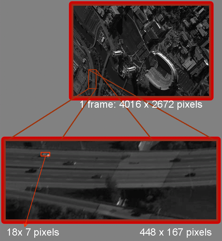
The problem that this project deals with is that of detection and tracking of large number of objects in Wide Area Surveillance (or WAS) data. WAS is aerial data that is characterized by a very large field of view. The particular dataset that we used for this project is the CLIF dataset. CLIF stands for Columbus Large Image Format, the dataset is available from [ https://www.sdms.afrl.af.mil/index.php?collection=clif2007].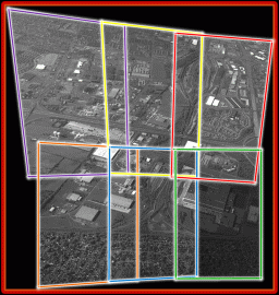 |
 |
 |
In CLIF, the sensor consists of six cameras with partially overlapping fields of view, mounted on an aerial platform flying at 7000 feet. All six cameras simultaneously capture 4016x2672 intensity images at 2 frames per second. Data obtained from such a sensor is quite different from the standard aerial and ground surveillance datasets, such as VIVID and NGSIM.
- First, objects in WAS data are much smaller, with vehicle sizes ranging from 4 to 70 pixels in grayscale imagery, compared to over 1500 pixels in color imagery in the VIVID dataset.
- Second, the data is sampled only at 2 Hz which when compared against more common frame rates of 15-30 Hz is rather low.
- Third, the traffic is very dense comprising thousands of objects in a scene compared to no more than 10 objects in VIVID and no more than 100 in NGSIM.
Method
The details of our method focus on tackling the issues that are peculiar to the WAS dataset.- Perform camera motion compensation using a point correspondence based alignment algorithm.
- Perform motion detection via a median image background model.
- We perform gradient suppression of the background difference image to remove motion detection errors due to parallax and registration.
- Divide the scene into a number of grid cells and optimally track objects within each grid cell using Hungarian algorithm.
- Link tracks across gird cells.
The following figure illustrates the overall pipeline of our method.

ALIGNMENT
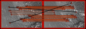
We detect Harris corners in frames at time t as well as at time t + 1. Then we compute SIFT descriptor around each point and match the points in frame t to points in frame t+1 using the descriptors. Finally, we robustly fit a homography Ht+1 t using RANSAC that describes the transformation between top 200 matches.

BACKGROUND SUBTRACTION
To perform motion detection, we first need to model background, then moving objects can be considered as outliers with respect to the background. Probabilistic modeling of the background as in [10] has been popular for surveillance videos. However, we found these methods to be inapplicable to this data. In the parametric family of models, each pixel is modeled as either a single or a mixture of Gaussians. First, there is problem with initialization of background model. Since it is always that objects are moving in the scene, we do not have the luxury of object-free initialization period, not even a single frame. Additionally, since the cameras move, we need to build the background model in as few frames as possible, otherwise our active area becomes severely limited. Furthermore, high density of moving objects in the scene combined with low sampling rate makes the objects appear as outliers. These outliers can be seen as ghosting artifacts as shown in figure below.
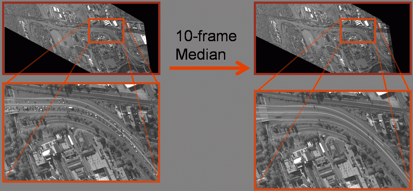
In the case of single Gaussian model, besides affecting the mean, the large number of outliers make the standard deviation high, allowing more outliers to become part of the model, which means many moving objects become part of the background model and are not detected. A mixture of Gaussians makes background modeling even more complex by allowing each pixel to have multiple backgrounds. This is useful when background changes, such as in the case of a moving tree branch in surveillance video. This feature, however, does not alleviate any of the problems we highlighted above. Therefore, we avoid probabilistic models in favor of simple median image filtering, which learns a background model with less artifacts using fewer frames. We found that 10 frame median image has fewer ghosting artifacts than mean image. To obtain a comparable mean image, it has to be computed over at least four times the number of frames which results in smaller field of view and makes false motion detections due to parallax and registration errors more prominent. We perform motion detection in the following manner. For every 10 frames we compute a median background image B, next we obtain difference image of the current frame from the background model.
GRADIENT SUPPRESSION
Prior to thresholding the difference image, we perform gradient suppression. This is necessary to remove false motion detections due to parallax and registration errors. Since we fit a homography to describe the transformation between each pair of frames, we are essentially assuming a planar scene. This assumption does not hold for portions of the image that contain out of plane objects such as tall buildings. Pixels belonging to these objects are not aligned correctly between frames and hence appear to move even in aligned frames. Additionally due to large camera motion, there may be occasional errors in the alignment between the frames.
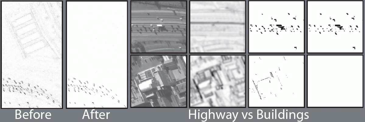
We suppress these by subtracting gradient of the median image (second column in the above figure) from the difference image. The top row shows a planar section of the scene and contains moving objects. As evident from figure 4, this procedure successfully suppresses false motion detections due to parallax error without removing genuine moving objects. Also, the method has the advantage of suppressing false motion detections due to registration errors, since they too manifest along gradients. Note that above method works under an assumption that areas containing moving objects will not have parallax error which is valid for roads and highways.
GRID AND OBJECT HANDOVER
After detecting moving objects, we track them across frames using bipartite graph matching. The assignment is solved optimally using the Hungarian algorithm which has complexity O(n3) where n is the number of nodes. When we have thousands of objects in the scene, an optimal solution for the entire scene is intractable. To overcome this problem, we break up the scene into a set of overlapping grid cells (as seen in the figure below).
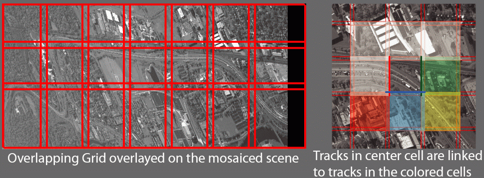
After tracking has been done within individual grid cells, we utilize the overlap of the cells to link the tracks accross cells.
TRACKING WITHIN CELLS
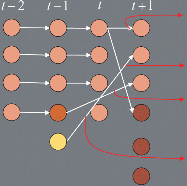
For each grid cell in every pair of frames we construct the following graph. Figure 5 shows an example graph constructed for assigning labels between frames t and t+1. We add a set of nodes for objects visible at t to the set of label nodes. A set of nodes for objects visible at t + 1 are added to the set of observation nodes, both types are shown in pink. Since objects can exit the scene, or become occluded, we add a set of occlusion nodes to our observation nodes, shown in red. To deal with the case of reappearing objects, we also add label nodes for objects visible in the set of frames between t-1 and t-p, shown in orange. We fully connect the label set of nodes to the observation set of nodes, using four types of edges.
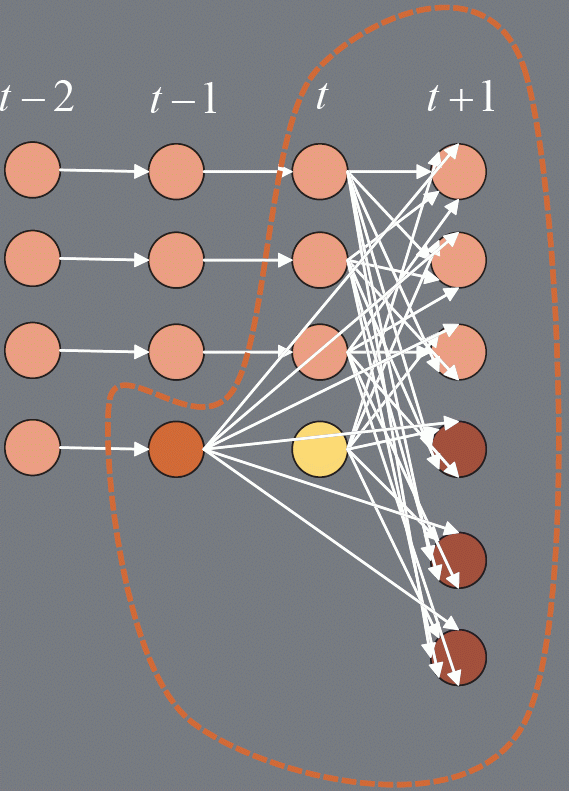
The graph contains four types of edges.
- Edge between label in frame t and an observation in frame t + 1 (pink node to pink node).
- Edge between label in frame t - p and an observation in frame t + 1 (orange node to pink node).
- Edge between a new track label in frame t and an observation in frame t+1 (yellow node to pink node).
- Edge between a label and an occlusion node (any node to red node).
 .
The edges of the fourth type are simply defined by a constant
  .
If the frame rate was much higher, or if the objects we are observing
were moving much slower, these two type of edges would be sufficient
for solving the tracker problem. Problem arises when a new object
appears in the scene since we do not yet have a velocity for that
object. Because of this we have to augment the weight of that edge
with various contextual information derived from the scene.
SCENE DERIVED CONTEXTUAL CONSTRAINTS
The first component is the road orientation estimate g. It is computed for each grid cell in the following manner. First, we obtain all possible assignments between objects in frame t and t+1. This gives us a set of all possible velocities between objects at frames t and t+1. Next, we obtain a histogram of orientations of these velocities and take the mean of orientations that contributed to peak of the histogram.
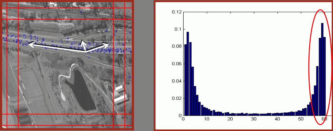
The road orientation component of the weight is computed as.

The second component is the formation context constraint. If we are trying to match an object in frame t (or t-k) to an observation in frame t + 1, we compute object context as a 2 dimensional histogram of vector orientations and magnitudes between an object and its neighbors. In order to account for small intra-formation changes, when computing the context histograms, we add a 2D Gaussian kernel centered on the bin to which a particular vector belongs.
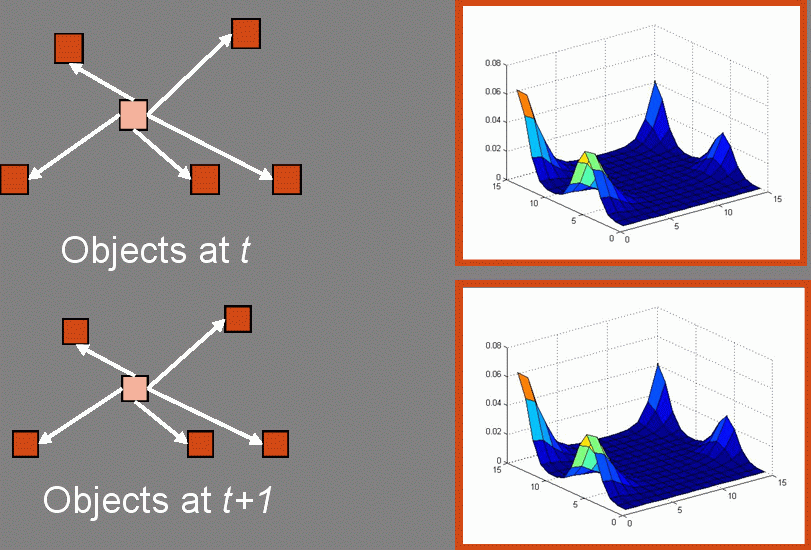
Furthermore, since 0 and 360 degrees are equivalent, we make the kernel wrap around to other side of orientation portion of the histogram. Compute weight as an intersection of two 2D histograms. Finally we compute the graph weight as follows.

The formal definition of all weights used is given in the figure below.
 |
 |
|---|---|
 |
|
 |
|
 |
MULTIPLE CAMERAS
Tracking across multiple cameras is handled in the following manner. We perform detection and tracking in global coordinates. We first build concurrent mosaics from images of different cameras at a particular time instant using and then register the mosaics treating each concurrent mosaic as a single image. One problem with this approach, however, is that cameras can have different Camera Response Functions or CRFs. This affects the median background, since intensity values for each pixel now come from multiple cameras causing performance of the detection method to deteriorate. To overcome this issue, we adjust the intensity of each camera with respect to a reference camera using the gamma function.

The cost function is minimized using a trust region method for nonlinear minimization. The approximate Jacobian matrix is calculated by using finite difference derivatives of the cost function. The intensity transformation is then applied to each frame of the camera before generating concurrent mosaics. Results for this procedure are shown in the figure above.
Ground-Truth
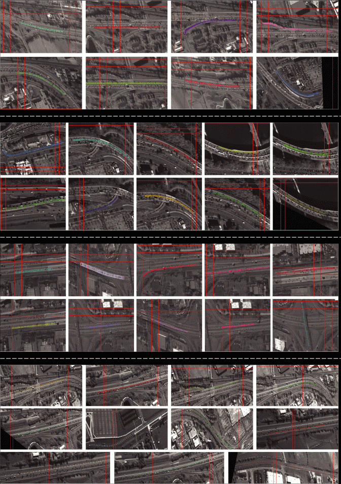
We have generated ground-truth for 4 sub-sequences of the CLIF dataset. The number of objects for which ground truth was generated are 34 for sequence 1, 47 and 60 for sequence 2 and 50 each for sequences 3 and 4. The rectangles in the figure below indicate the area in which the objects were ground-truthed.
[Download sequences information & ground truth here]
Experiments and Results
Quantitative Results
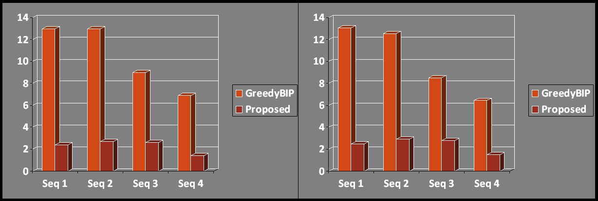
Quantitative measures of tracking performance consisted of Track Completeness Factor (TCF), Track Fragmentation (TF), and Normalized Track Fragmentation (NTF). To quantitatively measure detection we used Object Detection Rate (ODR). We compared our method against nearest-neighbor greedy bipartite graph (without constraints). The results are given below.

| |
Qualitative Results
[Download video for Sequence 1 here]