
[< Back to Home]
Learning Scene Model from Surveillance Videos
Downloads
Arslan Basharat, Alexei Gritai, and Mubarak Shah, Learning Object Motion Patterns for Anomaly Detection and Improved Object Detection, IEEE Conf. of Computer Vision and Pattern Recognition (CVPR), Anchorage AK, June 2008, [PDF]
Figure 6(a) has been updated in the latest PDF.
CVPR 2008 Poster [PDF]
Tracking Dataset [2MB ZIP] NEW!
Includes files:
- tower1_set1.txt (Tracks from a ~183 mins sequence)
- tower1_set2.txt (Tracks from a ~15 mins sequence, includes sitting,
unusual path, bicyclcist, skate-boarder, etc.)
- tower1_set2.avi (Xvid Codec) [54MB
Video]
- parseTrackFile.m (Matlab script to import tracks into track.mat)
Abstract
We present a novel framework for learning patterns of motion and size of objects in static camera surveillance. The proposed method provides a new higher-level layer, to the traditional surveillance pipeline, for anomalous event detection and scene model feedback. Pixel level probability density function (pdf)’s of appearance have been used for background modelling, but modelling pixel level pdf’s of object speed and size from the tracks is novel. Each pdf is modelled as a multivariate Gaussian Mixture Model (GMM) of motion (destination location & transition time) and size (width & height) parameters of the objects at that location. Output of the tracking module is used to perform unsupervised EM-based learning of every GMM. We have successfully used the proposed scene model to detect, not only local but also global anomalies, in object tracks. We also show the use of this scene model to improve object detection through pixel-level parameter feedback of the minimum object size and background learning rate. Most of the object path modelling approaches first cluster the tracks into major paths in the scene, which can be a source of error. We avoid this by building local pdf’s that capture a variety of tracks passing through. Qualitative and quantitative analysis of real surveillance videos proved the effectiveness of the proposed approach.
Our Approach
In this project we are developing a framework for abnormal event detection in surveillance videos. The abnormal events can be due to unexpected speed of objects, a person following suspicious path, cars violating one-way traffic, etc. The knowledge about the scene is used to improve conventional background subtraction.

Learning Scene Model
A scene model is learned using a set of training tracks. The proposed model is based on a combined Gaussian Mixture Model (GMM) of velocity (x,y,t) and size (w,h). A GMM is built for every pixel location to model the objects (tracks) passing through it. The use of GMM is important because it provides the strength of modelling multiple paths. We extract multiple transitions from each observation as shown in this figure.
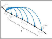
A set of observations with transition vectors between them are shown on a synthetic track. O_j and O_k represent two observations of the same object along the track. \gamma^k_j is the transition vector between O_j and O_k. Each one of these transitions forms a sample towards the learning of GMM. We rely on an EM based learning approach proposed by Jain et al. Details are available in the paper. Once the model has been learned, we have a GMM available at every pixel location, representing the pdf of normal tracks that have been observed during training phase. We use this model for following two problems:
Abnormal Behavior Detection
The learned scene model is used to detect abnormal tracks by checking the probability of each transition belonging to the pdf. Related equations and details are available in the paper. By using the higher order transitions we are able to catch global anomalies that can be very tricky and can easily blend-in as a normal track.
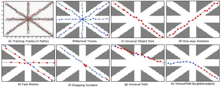
Synthetic scene four paths and various detected anomalies. Gray background is the region without motion model. (a) Training set of random unidirectional tracks (along four paths). (b) Shows randomly generated test tracks from the same normal distributions as for the training tracks. (c) A track with an unusual size as compared to the training sizes. (d) The training along the paths were done using only one-way traffic. If an test tracks violates that trend it can be easily detected by our system. (e) The speed violations can be detected using the same framework. Other abnormal events like an object stopping unexpectedly (f) and an object following an unusual path (g & h) are also handled by our approach. (h) A complicated anomaly can occurs when the tracks are not allowed to change paths, global analysis detects the violations. Every observation is labelled normal (blue diamond) or abnormal (red circle). Local analysis fails to identify anomaly, while global analysis highlights the observation that take unusual path.
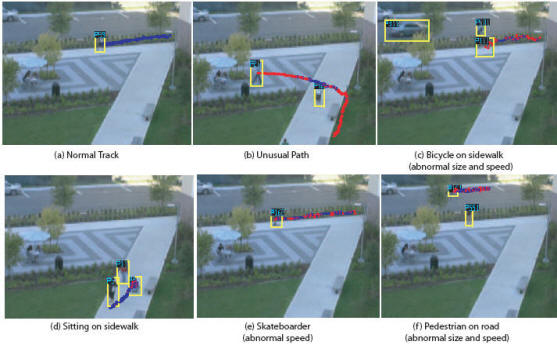
Detected abnormal observations are labelled red and normal ones as blue. (a) All normal observations of a typical pedestrian (b) Pedestrian follows an unusual path. (c) The observations from a bicyclist are also classified as abnormal because of abnormal speed and size of the object. (d) A person stops in the middle of the sidewalk and sits down. Note that the observations were correctly labelled normal before the person actually sat down. (e) A skateboarder, the size is the same as the pedestrian but speed helps in distinguishing. Some of the observations are detected normal because of only a slight difference in speed. (f) Unusual size and speed prove to be useful in case of a pedestrian walking on the road. All of the above mentioned tracks are part of the testing video which is separate than the training video.
Skateboarder on sidewalk
Pedestrian on road
Bicyclist on sidewalk
Unusual path followed by a pedestrian
Scene Model Feedback
Various parameters in the conventional background subtraction and tracking pipeline can benefit from the knowledge of the scene. These parameters are typically assumed to be constant throughout the scene. We show that the use of our scene model can improve the results by tweaking these parameters according to the knowledge about the scene. Following are the two parameters that we have used for the scene model feedback.
Parameter 1: Minimum Object Size
First parameter is the minimum size of the objects that are detected through background subtraction. This parameter is used to filter out noise, but you can miss real objects if they are very small. We use the learned pdf marginalized over the velocity parameters to model the typical sizes. This would give us higher probability for smaller objects only in the regions where we typically observe tracks of small objects. Following figure shows and illustration of the size map generated from the marginalized pdf. See papers for the details.
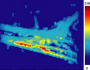
The object size map is computed for scene shown below. Intensity at every pixel is the most probable size of the object observed at that location. The highest intensity (biggest size) is observed for the vehicles along the road. Note the gradually reducing sizes due to perspective effect.
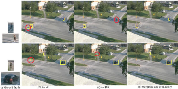
Improvement in object detection by the proposed size model. Each row presents an instance in the same video. Column (a) shows the manually extracted patches of the objects currently present in the scene. Column (b) is the output when a uniform global value of s = 50 is used. Noisy foreground blobs are also detected as valid objects (red ellipses). (c) presents output when s = 150 throughout the scene. Individuals are not detected (red ellipses) when the object size is small. (d) presents results of the proposed size model. In both scenarios the valid objects are detected and the noisy observations are avoided.
Parameter 2: Background Learning Rate
Second parameter that we improve using the scene model feedback is the background learning rate. A constant value is typically used for the complete scene and this can cause problems when objects start stopping for longer than usual. One cannot reduce the background learning rate for the complete scene to address this problem as this would make the system less adaptive of the sudden illumination changes. We marginalize the learned scene model pdf's over the size (x,y) paramters and highlight the exit locations in the scene. The learning rate is then posed as a function of the probability of the reducing velocity of the object. See paper for the derivation and the details. We show one scenario here when the car stopping at the traffic light is learned as a part of the background at the usual learning rate.
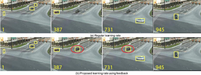
Improvement in object detection using the proposed feedback approach for updating learning rate. Video sequence progresses from left to right. (a) Using the uniform background learning rate (\rho = 0.01) for the whole scene. (b) Detection results using the proposed approach for updating background learning rate. Red ellipse highlights the detection of stationary car that was missed by the regular approach.
[< Back to Home] [^ Back to Top]