City Scale Geo-spatial Trajectory Estimation of a Moving Camera
- Related Publications
- Problem Definition and Overview
- Proposed Method
- Test Videos
- Experiments and Results
Related Publications
"City Scale Geo-spatial Trajectory Estimation of a Moving Camera".
Gonzalo Vaca-Castano, Amir Roshan Zamir and Mubarak Shah
IEEE International Conference on Computer Vision and Pattern Recognition(CVPR), 2012. [PDF]
"Accurate Image Localization Based on Google Maps Street View".
Amir Roshan Zamir and Mubarak Shah
European Conference on Computer Vision (ECCV), 2010. [PDF]
Problem Definition and Overview
In this work, we address the problem of extracting the geospatial trajectory of the camera from unconstrained videos recorded in a city. The proposed method is intended for user-uploaded videos available on the web, which typically include undesired recording defects, such as blurred or uninformative frames, abrupt changes in camera motion, zooming effect, dynamical environment of the scene such as vehicles and pedestrians occluding distinct features, and lack of information of the initial position and pose (e.g. meta data) where the video was recorded.Proposed Method
The steps of our method for estimating the trajectory of a moving camera in a city are despited in the next figure:
 |
| |
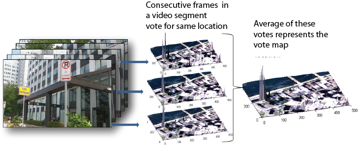
Frames are sampled periodically from the video. Each frame of a video is geolocalized, with the help of a reference dataset of Street View images with GPS placemarks, according to the procedure described in our previous work . The output of the individual frame geolocalization algorithm is a probability map with votes over the most probable locations. In our previous work, the highest peak in the probability map of votes is selected as the GPS location of a query image. However, the same technique fails in videos because sequences typically contain many frames that are not assigned to the correct geolocation.
VIDEO SEGMENT GEOLOCALIZATION
The GPS placemark locations in the reference dataset are spaced approximately every 12 meters. All the sampled frames from the query video corresponding to the time period where the camera moves 12 meters around a placemark, should vote for the same location in the reference dataset. This can be interpreted as a quantization process since we are constraining a continuous set of values (global position) to some discrete set of values (GPS placemarks). Processing individual frames will produce a quantization error in the frame position estimation. Therefore, it is more helpful to gather sets of consecutive frames and treat them as a video segment. Hence, a map of votes corresponding to a video segment is achieved by averaging the vote maps of each one of the frames that belong to the segment.

BAYESIAN FILTERING
A Bayesian formulation is plausible, if the vote distribution of the video segment is interpreted as the likelihood of the location (latitude and longitude) given the current observation. A video is constrained in the spatial and temporal domain because consecutive frames correspond to close spatial locations. Consequently, Bayesian tracking is used to estimate the frame localization and its temporal evolution. The objective is to estimate the state x (latitude and longitude) at any sampling time t. To do this, we need to calculate the probability of the state x given the previous history of observations Z. Using bayesian theorem and under the Markov assumption, the following expression can be derived:


The normalization constant is a measure of how often the number of votes estimated in the current state is close to the probability predicted from the previous state (gate). In other words, a value c close to zero could indicate false localization. Therefore, the value of the variable c is used to discard some of the untrustworthy observations. The state estimation in cases where c is close to zero are discarded, and a new probability function is built using the earlier state estimation as the most probable state. In the case that the value of c is close to zero in several consecutives estimations, a redetection process is performed, the same way the initial geolocation is computed, as described below. In the case where the values of c are not close to zero, the estimation of the state would be given by the expectation.
Our experiments show that the constant velocity motion model performed slightly better than the constant acceleration and random walk/Brownian motion models in our method.
Initial Geolocalization
In order to obtain the initial geolocalization, we consider a group of periodically sampled frames around the first frame of the video. For each one of the sampled frames, its frame geolocalization is estimated as the highest peak of the vote distribution of the frame. It is highly probable that some of these frames are not correctly geolocalized; therefore, we have used two different pruning steps to remove them. The first step is to reduce the number of false geolocalizations using the information provided by the Confidence of Localization (CoL), which was used in our previous work. The estimated frame geolocalization is discarded by thresholding the CoL value. The second step is to discard the geographically isolated frame localizations by counting the number of frame geolocations within a prudent radius r of the frame being tested. The frame is discarded if the number of surrounding neighbors is less than the threshold. After applying these two pruning steps, the remaining frames are averaged to obtain an estimation of the initial geolocalization.
MINIMUM SPANNING TREE-BASED TRAJECTORY RECONSTRUCTION
Any on-line (causal) approach to enforcing temporal consistency which exploits a motion model poses some "inertia" in motion estimation. Additionally, any scale image localization method which provide the input to the Bayesian Filter, are expected to geolocate a frame with an error of a few tens of meters. Although this error value is acceptable for a city scale localization algorithm, it can cause inconsistency in the trajectory that the video segments form, even after applying the Bayesian filter. Therefore, we propose a trajectory reconstruction method based on Minimum Spanning Trees which can effectively handle these complications.

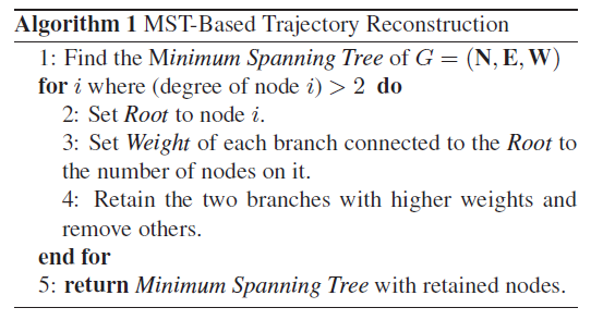
The process of MST-based trajectory reconstruction is illustrated in next figure. First, the output locations of the video segments and their respective time (a)) are acquired from the Bayesian Filter and the graph G is formed. Then, the Minimum Spanning Tree of G is found (b). The degree of a node in a MST is defined as the number of edges connected to it. The next step is to identify the nodes with a degree higher than two (orange nodes in figure (b)). For such nodes, we define the weight of each connected branch as the number of nodes connected through that branch to the root. This is illustrated in figure (c) for one of the nodes with a degree higher than two. Then, the nodes on the two branches with the highest weights are retained and the rest are removed. When a node with a degree higher than two is observed, it means there is a node which is likely off the mainstream of the trajectory and consequently an additional branch has appeared. Such a node is either geospatially or sequentially inconsistent with the rest of the path. The process of assigning a weight to each branch is intended to identify the branch(es) which contains an outlier and consequently should be removed. The branch which has fewer nodes that are connected to the root is less likely to be on the mainstream, since fewer video segment locations are consistent with its location. Therefore, we retain the two branches with highest weights, which ensures the connectivity of the trajectory, and remove the rest. The final trajectory is shown in figure (d). Note that the features used to determine the MST, include both time and geolocation information. Therefore, if the camera revisits a previously visited location, the nodes corresponding to the first and second visit will not be mistakenly linked in the MST as their time features are very different even though their geospatial locations are close.
 |
| Illustration of the different steps of MST based trajectory reconstruction. The green trajectory represents the ground truth. a) Output of the Bayesian filter. b) Minimum Spanning Tree. The nodes with a degree higher than two are shown in orange. c) The branches of a particular node with a degree higher than two (shown in orange) are marked with arrows. Yellow and purple branches are retained and the blue one is removed as it has less weight. d) The final reconstructed trajectory. |
Test Videos
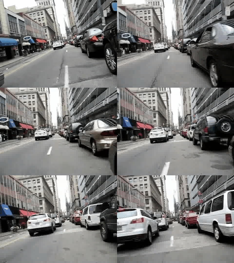
We have tested the proposed algorithm on a data set of 45 videos, with the durations ranging from 60 to 120 seconds and total number of 106,200 frames. The query videos are from downtown Pittsburgh, PA and downtown Orlando, FL; they were downloaded from YouTube or recorded by different users using a consumer grade video cameras while walking or driving in the city without prior knowledge about the usage of the videos.
[Download test video sequences & ground truth here]
Experiments and Results
Quantitative Results
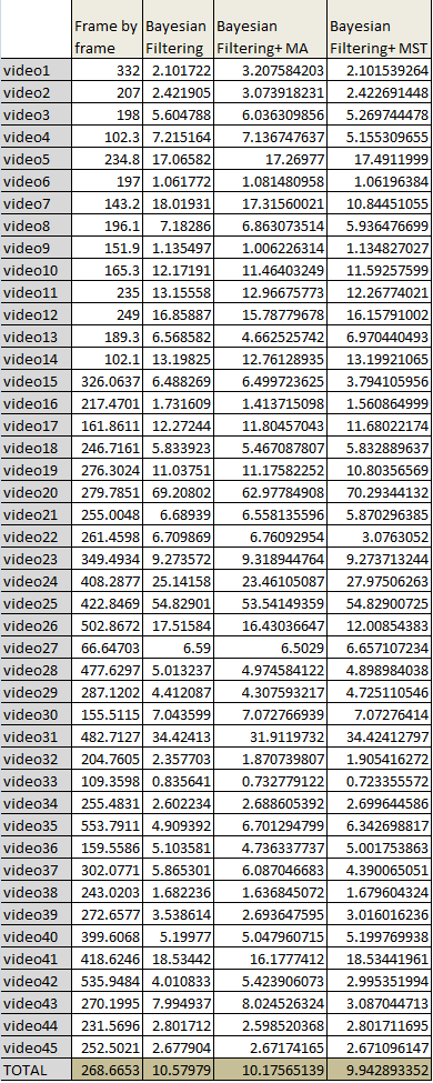
Quantitative measures of mean error in meters are presented for the 45 test sequences. The first column of the table contains the results obtained using individual frame by frame geolocalization. Mean errors of individual frame by frame geolocalization of these videos range from 66 to 535 meters. These values demonstrate the low performance of frame by frame geolocalization in determining a trajectory. The mean errors of the proposed Bayesian filter is found in the second column. The mean errors in most of the videos are lower than 20 meters. The subsequent rows in the table compare the trajectories obtained after applying moving average (MA) smoother to the output of the Bayesian filter versus the trajectories obtained using the proposed MST based trajectory reconstruction applied to the output of the Bayesian filter. As can be seen, most of the best results correspond to the MST-based trajectory reconstruction method.

Qualitative Results